You Too Can Use Excel Like A Pro – Here’s Part 2 of Our Series to Show You How

With the 2016 version of Excel, Microsoft has really upped its game for people who aren’t great with numbers. You can now easily use one-click access that can be customized to provide the functionality you need.

This is the second of our three-part series about using Microsoft Excel 2016 to help you identify trends, construct helpful charts, and organize information to maximize the value of your data.

 

Did you know that you can use Excel Worksheets and Workbooks in conjunction with programs like Microsoft Access and PowerPoint? Excel 2016 possesses many capabilities that aren’t readily apparent. That’s why we’re providing this three-part series for you.

If you missed Part 1 of our series, you can find it on YouTube at:

In this, Part 2 of our series we’ll be discussing:

• Working with Multiple Worksheets and Workbooks
• Managing Lists
• Working with Dates
• Formatting and Conditional Formulas
• The IF, AND and OR Functions

Why would you want to use Excel?

If you or your employees work with financial data, it’s a great tool to use for:

• Basic mathematical operations like adding, dividing, and multiplying.
• Finding values like profits or losses.
• Calculations like averages, percentages and number counts.

Performing calculations in Excel is only the tip of the iceberg. There’s much more you can do like creating charts and graphical layouts to make it easier to recognize trends and more easily analyze data.

What is Excel and how is it organized?

Excel is an electronic spreadsheet program that’s used to store, organize and manipulate data. You enter data into Workbooks that are made up of individual Worksheets. In the Worksheets, you enter data into cells that are organized into rows and columns. Excel data can consist of text, numbers, dates, times and formulas.

Working with Multiple Worksheets and Workbooks

Before you build your worksheets and workbooks think through the process and ask yourself:

“How do you want to see and analyze the results?”

“How much detail is needed to draw a conclusion?”

“What is the most important data for decision makers?”

To access or create a Worksheet, go to the tabs at the bottom left of the screen and click the one you want to activate. Or use Control Page Up or Control Page Down to move among your Worksheets using the keyboard.

You can move or copy a worksheet by going to the tab, right-clicking, and you’ll be presented with a dialog box where you can select your function. You can move your worksheet to a different Workbook by entering its name in the space above.

Use the scrollbars on the right to make other selections like making a copy. Simply click the checkbox for the action you wish to take.

Working with Formulas Across Worksheets

You can calculate different formulas across a worksheet with what Microsoft Excel calls 3D formulas. 3D formulas allow you to calculate data throughout a workbook using multiple worksheets. It refers to the same cell (or range of cells) on multiple worksheets.

Think of a 3D formula as a cross-reference to data in a different Worksheet.

It’s a great way to build summaries and Master Worksheets to bring them together in one place. And it’s a must if your labels and data types vary between worksheets.

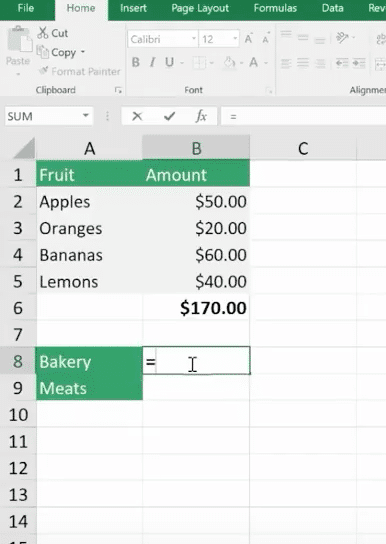
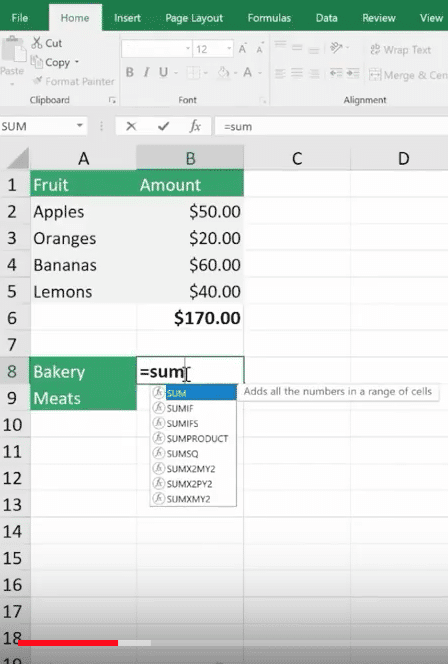
Here we want to bring in the formula from another worksheet to this one. We have three worksheets for our inventory costs. We have a breakdown for our Fruits Dept. But we want to bring in the costs for our Bakery and Meats. So, we go to the cell we’ve created, select =sum, hit the left parenthesis ( then navigate to the Bakery Worksheet tab at the bottom, click on the cell where we want the formula to appear and hit Enter. Then the inventory cost automatically appears.

All 3D formulas are based on this syntax: Sheet1:Sheet4!A2:B5.
If you copy or insert a new worksheet after Sheet1 the reference will automatically include it.

Similarly, if you delete a worksheet it will be excluded.

Consolidate Data

You can consolidate data from separate worksheets into one Master Worksheet. They can be in the same workbook or from other Workbooks. Let’s say you have a sales team and a worksheet with their weekly report data, and you want to consolidate this data into a monthly report. There are two ways to consolidate this data:

1. Consolidate by Position: This is when the data in the source areas is arranged in the same order and uses the same labels. You use this method to consolidate data from a series of worksheets that have been created from the same template.

2. Consolidate by Category: Use this method when the data in the source areas is not in the same order but uses the same labels. Here you consolidate data from a series of worksheets that have different layouts but have the same data labels.

We are only going to demonstrate Consolidate by Position because it’s an organizational best practice.

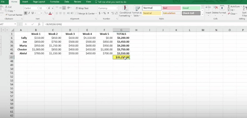
Here’s our example Workbook. Data is in the same order and uses the same labels.

Creating a clean master worksheet for this is best. But if you use a worksheet with pre-existing data make sure you have a blank area where the consolidated data can appear.

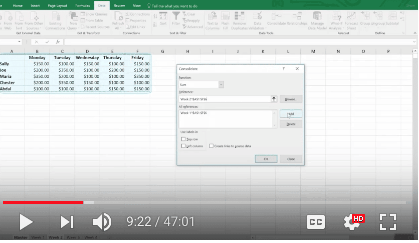
To start, click in the upper left-hand corner and click Consolidate. A window will open. By default, SUM will be your option, although there are others to choose from. Average is the next most common function people use.

Now we want to choose our ranges from each of the worksheets. We’ll collapse the Consolidate box and click on Week 1. Select the entire range.

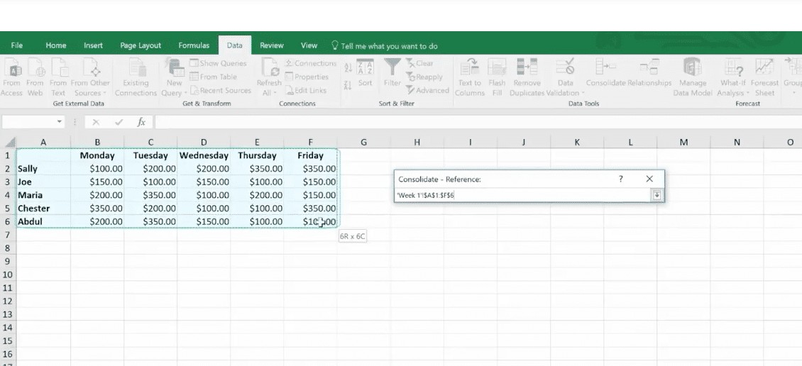
Bring back the dialog box and add this week to the references.

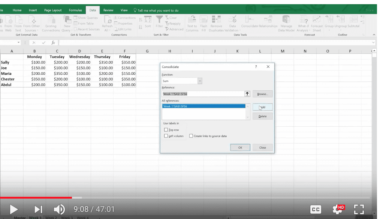
Now, when you click on week 2 to do the same, it’s already pre-selected. Just click Add. And do the same for the next two weeks. Now you’ve told Excel what data you want to consolidate.

Creating Links

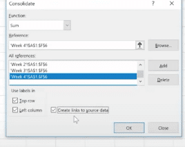
You must choose between automated and manual updates. If you want Excel to consolidate your worksheets automatically when you change data, you must tell it to do so by checking this box: “Create links to source data.”

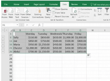
Press OK and Excel will generate the consolidation. It’s up to you to format it the way you want. But you’ll only have to do this once if you used “create links.” If so, Excel automatically updates any changes.

Notes:

You can’t create links if the source and the data are on the same worksheets. This means it’s smart to group data into worksheets in smaller periods. In this case, we did it by weeks.

If the information you want to consolidate is in a different Workbook, you want to browse for that Workbook before you begin the consolidation process. Then you can select the reference in the same way we did above. Excel will create the path for you.

Linking Workbooks

Up to this point, we’ve been working in one Workbook with several worksheets. Just like we pulled data in from multiple worksheets, we can do the same with multiple Workbooks.

Remember our 3D formula? When this same type of linking crosses over to a different Workbook it’s called an “External Reference.” Sticking to our Sales worksheet example, you may have a Workbook for each month or each year.

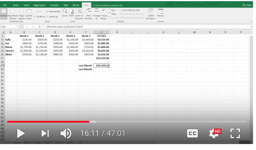
We now want to compare how our Sales Team did month to month instead of week to week. We are going to add a link to last month’s total. Just like before: select =sum, hit the left parenthesis ( and navigate to the Workbook you want. (Here’s it’s the Monthly Sales Workbook.)

You’ll see that single quote marks have been added to the syntax. This is because there is a non alpha-numeric character in the name (space). You’ll need these when links are broken as well.

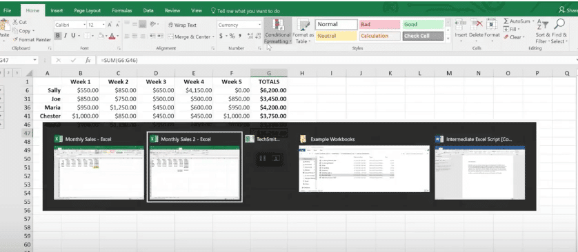
Here’s how to do it in the opposite way. Start in your first file, go to copy or Control C.

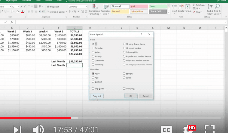
Go back up to Conditional Formatting and grab your Workbook and do a “Paste Special.”

And down at the bottom left click “Paste Link.”

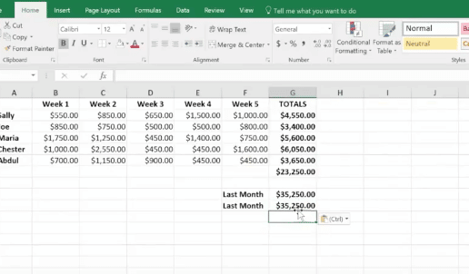
And here it is.

Managing Lists

Excel lists don’t typically use formulas. They use filtering and sorting instead. So, it’s important that lists have column headings and that there are no empty rows in your lists.

First, we’ll do a simple sort: From the list below, we’re going to organize who had the most wins.

• We click the column header for Wins.
• Go up to Sort & Filter in the top right and sort from highest to lowest.

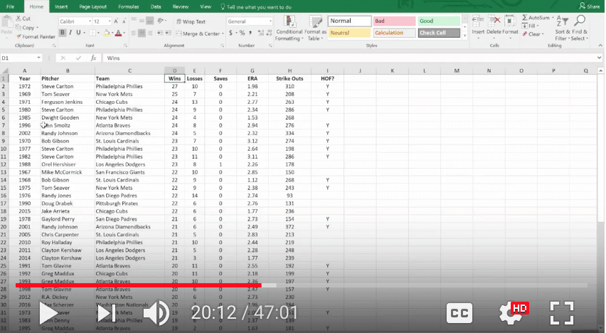
Next, we’ll sort by multiple columns:

Select your columns.

Go to Sort & Filter > Custom Sort

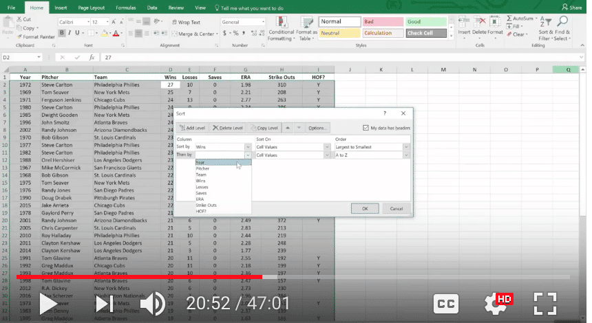
And we’re going to sort by Earned Run Average (ERA).

You can see below that it worked. (ERA sorts smallest to largest because a smaller number is better.)

Auto Filtering

This is how you can include or exclude any row data.

Select any column or header and under Sort & Filter choose Filter.

To the right of any column header there’s a drop-down menu.

We’re going to see who was selected for the HOF (Hall of Fame.)

Click the drop-down and deselect everything.

Then choose Y (for yes).

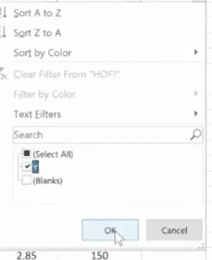
Click OK and now you’ll see just the players who were selected for the Hall of Fame.

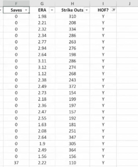
The Filter Icon is an easy way to see that a column is filtered.

Now we’ll customize the filter by Strike Outs.

Click the drop-down next to Strike Outs.

Choose Largest to Smallest.

And now the list is ordered by Strike Outs.

We want to see how many Wins they had. Go to the Wins and click the drop-down menu. Under Number Filters.

Choose Less Than and enter 20 > OK

Now we see the pitchers who won less than 20 games.

Sum Up Totals

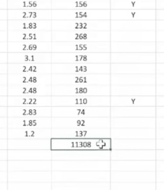
Click in the cell where you want the Sum to appear and choose AutoSum>Enter.

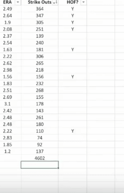
And if you decide to take off all the filters, the Sum will recalculate automatically.

Working with Dates

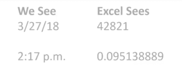
Dates and times are the most common functions people work within Excel, but they can be frustrating because Excel uses a serial number to represent a date instead of the typical 01/02/18 format and hours, minutes and seconds that we’re used to. It’s further complicated because dates are days of the week.

For example, In this system, the serial number 1 represents 1/1/1900 12:00:00 a.m. Times are stored as decimal numbers between .0 and .99999, where .0 is 00:00:00 and .99999 is 23:59:59. The date integers and time decimal fractions can be combined to create numbers that have a decimal and an integer portion. For example, the number 32331.06 represents the date and time 7/7/1988 1:26:24 a.m.

The Date Function will help. It’s on the Formula part of the Ribbon under Date & Time.

The TODAY() Function and the NOW() Function

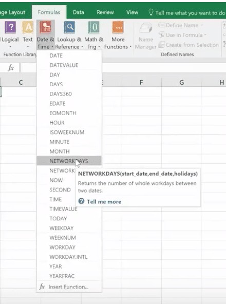
The TODAY function returns the serial number of today’s date based on your system clock and does not include the time. The NOW function returns the serial number of today’s date and includes the time.

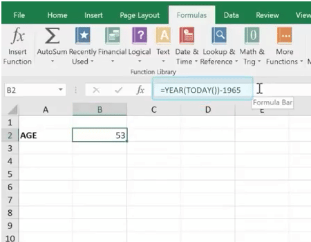
Here we are using the Today function. Excel will always use the exact date. The Today function is useful for calculating intervals. You might use this function to calculate someone’s age.

For example, we entered =YEAR(TODAY())-1965

And the age Excel came up with is 53.

TODAY always had the () following it.

The NOW () function is useful when you need to display the current date and time on a worksheet or calculate a value based on the current date and time, and want that value updated each time you open the worksheet.

Formatting Dates

This is found on the Home Ribbon.

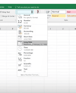
Under DATE you can see many ways you can display your information.

Formatting and Conditional Formulas

Conditional formatting highlights important information in a spreadsheet. But sometimes the built-in formatting rules aren’t enough. Adding your own formula to a conditional formatting rule helps you do things the built-in rules can’t do.

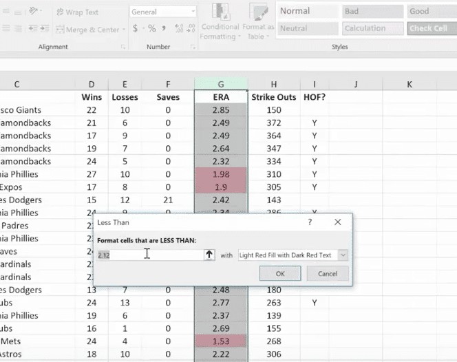
Here we want any ERA lower than 2 to be highlighted in red.

Highlight the column and click on Conditional Formatting.

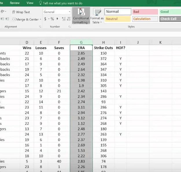
We selected Cells Less Than 2.00

The IF, AND, and OR Functions

IF

The IF function helps you make logical comparisons between a value and what you expect. For example: IF(Something is True, then do something, otherwise do something else)In this sense an IF statement can have two results. The first result is if your comparison is True, the second is if your comparison is False.

Below we’re going to determine our WINNER based on a calculation of IF:

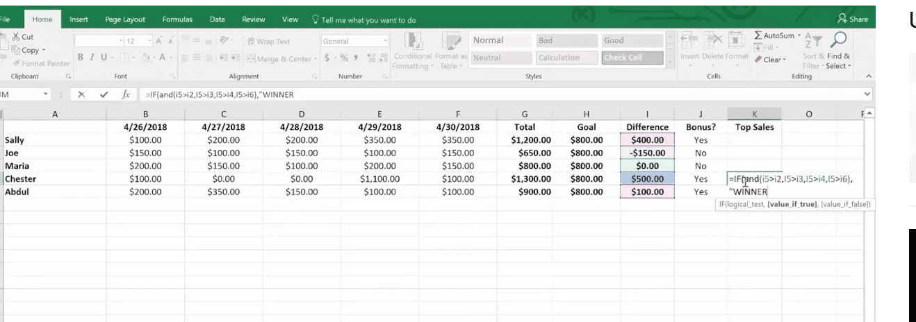
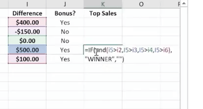
Based on our IF formula, Chester is our WINNER!

OR

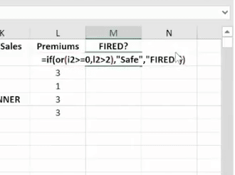
Use the OR function, to determine if any conditions are TRUE.

Here we use a formula that tells us if someone is SAFE or FIRED.

That’s it until next time! To View this Demo on YouTube visit: